Excel Tutorial – Filtering your data

Add a filter to your column headers

As we saw at the end of the section on sorting, to add the filter option to your columns, you can:

Use the keyboard shortcut Ctrl + Shift + L
Or click the Data tab > Filter

With this action, you now have arrows for each column header.

How to apply a filter

Filtering data is simple and intuitive.

Click the arrow in the column where you want to apply a filter
Uncheck all items
Select the item you want
Click OK

How to filter on a single value from the headers

Then, only the selected item is visible in your spreadsheet.

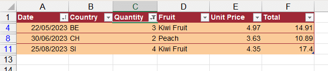
It is important to note three things:

When a filter is applied, the row numbers are blue
The filtered column has a specific icon
The other rows aren't deleted, just hidden

Filter from spreadsheet data

Another way to filter your data is with the right-click. For example, to filter on country CA, simply:

Select a cell that contains the word 'CA'
Right-click
Select the menu Filter
Then Filter by selected value

As you can see, you can filter on:

a specific value
a background or font color
an icon (from conditional formatting)

But you can't filter on numeric values larger than or smaller than this way.

Filter on numeric values

When the column contains numeric values, new filtering options are available:

Open the Filter dropdown
Select the Number Filters option

In the upper part (red box), we have the standard options for selecting numbers (greater than, smaller than, between...)
In the lower part, we have more elaborate filtering options (Top 10, Above Average)

You can also choose to display only the top 5 values in the dialog box.

Worked example: filter for values greater than 30

We want to select all sales greater than 30.

Which option was chosen to achieve this result?

Filter on Dates

Applying a Filter on a date is one of the most interesting filtering options. When you open the Filter pane, you see only the years, not all the data.

Clicking the + in front of a year expands the months, then the days. This way, you can very easily select an extremely precise time period.

However, the Filter on a date option also allows you to spot lines with incorrect dates (like here, 12/16/2022). Because the date doesn't exist, it isn't included in the automatic date breakdown. Instead, it's displayed separately as a text value.

Chronological Filter Option

When you have dates in a column, the menu shows you the option Chronological Filters. This option is much richer than the one for numeric data, because it gives you a breakdown by day, week, month, quarter, and year.

Filter on a color

Just like with sorting, you can filter by color — and it's super convenient! 😀😁👏

For example, in the following situation, to filter on yellow-colored cells, simply:

Click the filter option in the header
Select the Filter by Color option
Select the color you want (Yellow)

Then only the yellow cells are visible. Also, the filtered rows are blue, and the filter icon shows as active.

You now know how to filter your data by value, by number, by date, and by color — and how to make sure the rows you don't see are only hidden, never deleted.

Continue learning

Keep building your Excel skills with the rest of this tutorial series: