Adjust column width manually
To expand or reduce a column's width, follow these steps:
- Position your cursor between two columns
- The cursor changes to a long line with two opposite arrows
- When this cursor appears, click the mouse button
- Hold down the mouse button
- Drag right to expand the column, or left to collapse it

Manually adjust several columns in a single action
To save even more time, you can change the size of several columns in a single operation.
- Select several columns (like A to E in our example)
- Position the cursor between two of the selected columns (it doesn't matter which ones)
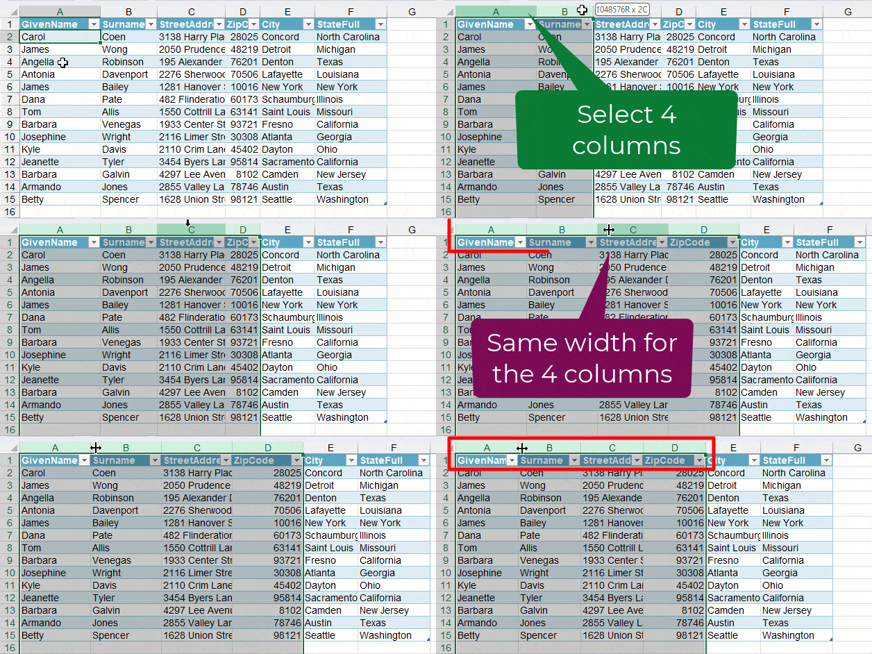
- Apply the click-and-drag technique to obtain a width of 80 pixels
- When you release the mouse button, only the selected columns are resized
Fit a column exactly to the widest content
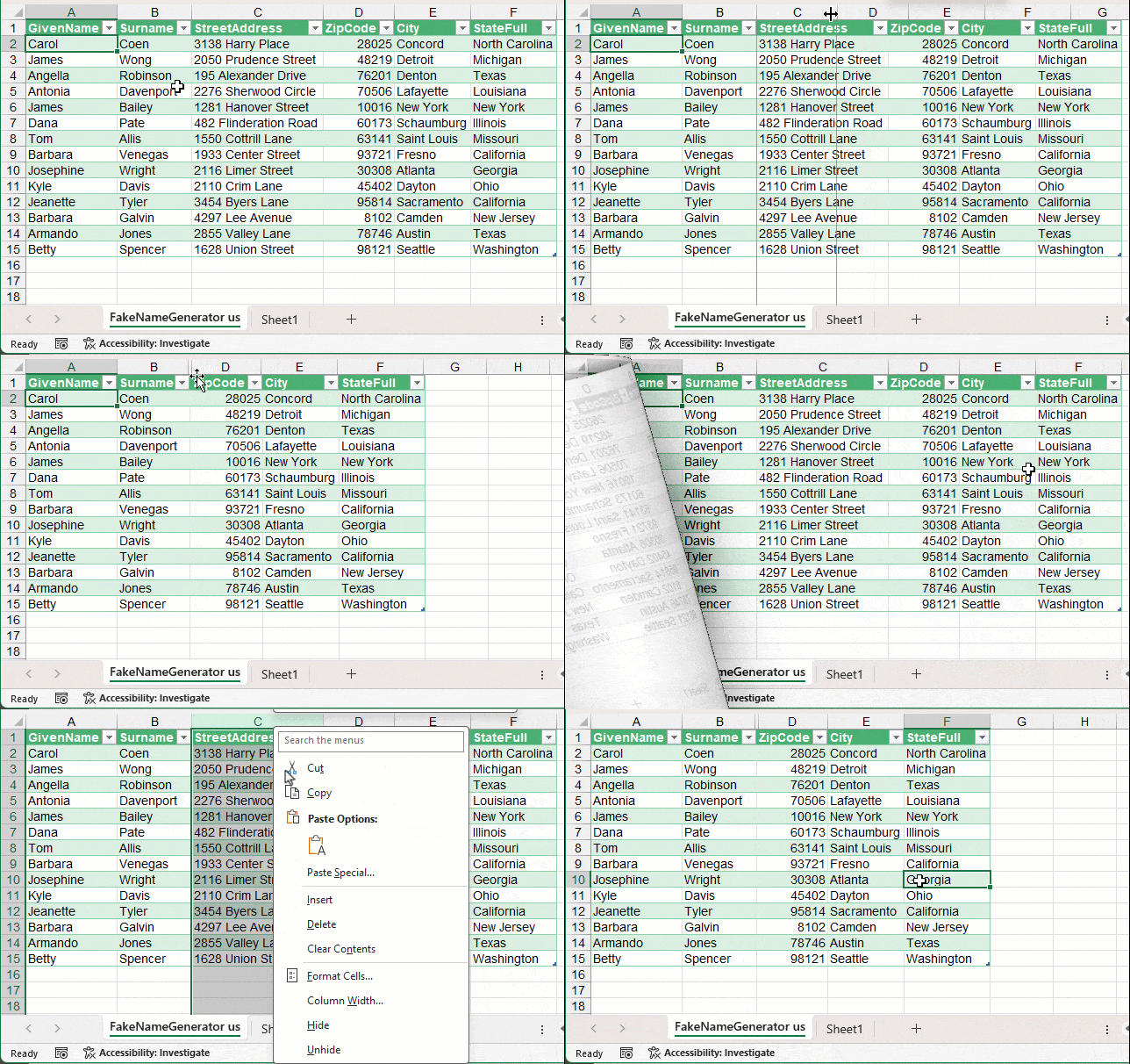
There's a very simple trick for fitting a column's width exactly to its widest content. Here, we want to adjust the width of the address column (column C).
- Place the cursor between columns C and D
- Double-click when the double-headed arrow cursor appears
- Excel automatically adjusts the width to the broadest content (in this case, row 7)

Fit several columns exactly to the widest content
The same trick works if you select several columns at once.
- Select several columns, here from A to D
- Place the cursor between two of the selected columns (it doesn't matter which one)
- Double-click when the double-headed arrow cursor appears
- Excel automatically adjusts the width of the four selected columns

Hide columns
Excel lets you hide the contents of a column. Two techniques are possible:
- Reduce the width of the column to 0 pixels
- Right-click in the column header and select the Hide option
Show a hidden column
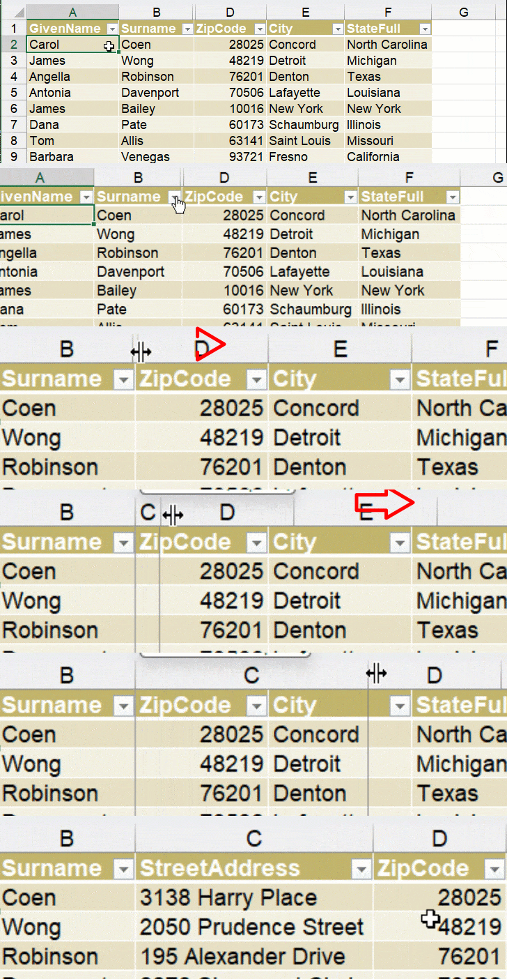
Note the double line between columns B and D, indicating a hidden column.

To show a hidden column with the mouse:
- Place the cursor on the column marked with the double line
- Wait until the cursor shows the double-line icon (the arrows stay inverted)
- Click and drag to unhide the column
Continue learning
Keep building your Excel skills with the rest of this tutorial series:
- Tutorial - Excel keywords
- Tutorial - How to make calculations in Excel
- Tricks to Insert, Delete, Hide Rows and Columns
- Tutorial - All Excel tricks to Copy-Paste
- Tutorial - Moving cells or columns with the mouse
- Tutorial - The Numbers Format
- Tutorial - Excel Alignment text tips
- Learn the secrets of Sorting Data with Excel
- Excel Tutorial - Filtering your data
- Manipulate Text in Excel without formula
- Excel Tutorial - Creating a dropdown menu
- Learn how to use the SUM function in Excel
- Tutorial for the Excel Functions AVERAGE, MIN, and MAX
- Learn how to use the Dollars in an Excel formula


