Excel Tutorial
Excel tutorials, quizzes & AI guides — all levels
RSS
  • Online Excel Exercises
  • Excel Tutorials
  • Excel Tests
  • Sitemap
  • Premium Quizzes
  • Shop
  • My account

Learn how to use the SUM function in Excel

Simplify your formula

In the previous module, we saw how to build a formula.

But if you need to add many cells, building a formula like =B2+C2+D2+E2+F2 causes real problems:

  • It takes a very long time to select each cell 😡
  • It's a common source of errors — easy to forget a cell đŸ˜±
  • Formulas like this are difficult to maintain đŸ˜€
Add many cells one by one is not a good solution

The SUM function solves this: it adds up multiple values across many cells in one go. Just follow these steps:

  1. Write =SUM
  2. Then open parenthesis
  3. Select the range of cells to add: B2:F2
  4. Close parenthesis
  5. Press Enter
SUM function to simplify the way to add many cells

The result is exactly the same — but the formula was much simpler to build 😀 👍

Copy the SUM

When you copy the formula using one of the methods shown in this tutorial, the sum is calculated for each row individually.

Copy the SUM function for all the other rows
  • Here, the formula was copied downward.
  • So each reference's row number increased by one.
  • This way, you only need to write the formula once for the whole sheet.

Example: sum for Monday

What formula should you write to calculate the sum for Monday?

Question how to calculate the sum for Monday

To calculate the total Monday sales, select the range containing all sellers' sales, such as B2:B9.

Answer to calculate the sum of Monday

Copy the SUM function for the other columns

Copy the formula to the right again to get the sum for each day of the week — this time, the column references change in the formulas.

Copy the SUM function to the right for the other columns

Shortcut to call the SUM function faster

The SUM function is used so much in Excel that it can be called from the ribbon or by keyboard shortcut.

From the Ribbon

  1. Select the cell where you want the total to appear — in this example, B10
  2. Click the ÎŁ icon (AutoSum) from the Home tab
Create a sum with the Autosum button

Clicking the ÎŁ symbol does the following:

  1. Selects all cells with numbers (excluding text and empty cells)
  2. Displays the function in the formula bar
  3. Press Enter to validate the result
Create a sum with the shortcut alt =

Keyboard shortcut

Instead of clicking the Σ symbol, you can get the same result with the keyboard shortcut Alt+= 😉

Use the Quick Analysis tool to do a SUM

Quick Analysis is the name given to the icon that appears after making a selection in your spreadsheet.

Excel quick analysis tool
  1. Select all cells with numbers
  2. The Quick Analysis icon is displayed at the bottom right
  3. Select the menu Totals
  4. Finally, select the Blue Sum option (the icon has the symbol ÎŁ and a blue line for the Total)
Option Total in the Quick Analysis tool

 The sum of all columns is instantly calculated and added to the row below the selected range.
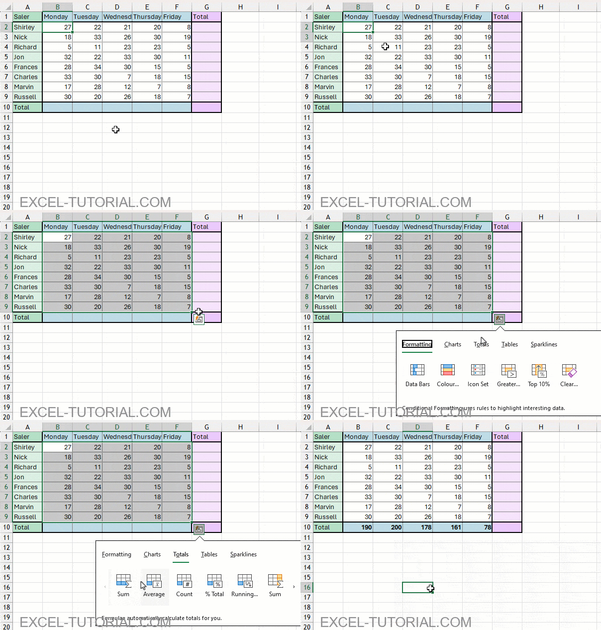
Sum of the rows with the quick analysis tool

Same trick for rows

Now, if you want to sum all the cells of the same row, the technique is the same.

  1. Select the cells you want to add
  2. Click the Quick Analysis icon
  3. Go to the Totals tab
  4. Select the Yellow Sum option (symbol ÎŁ and a yellow column for the Total)
Quick analysis to perform a sum for the rows

The result is as follows.

Sum by row with the quick analysis tool

Now practice it yourself

Time to put the SUM function to work on a real case: calculate a week of ticket revenue, full-price and half-price, day by day, then the grand total for the week.

Weekly revenue calculation

Calculate a week of ticket revenue from full-price and half-price customers: unit totals with absolute references, row totals, then SUM and AVERAGE — 10 guided steps.

The full-price reference must be locked.

1 / 10

Write in D2 the formula to calculate the full-price amount.

Revenue — Q1 · 474

=B2*$C$11

The $C$11 rate stays locked, the B2 reference shifts down.

2 / 10

Fill the formula down from D2 to D6 using the fill handle.

Revenue — Q2 · 475

=B6*$C$11

The half-price ticket rate must be locked.

3 / 10

Write in E2 the formula to calculate the half-price amount for Monday.

Revenue — Q3 · 476

=C2*$C$12

Same as column D: $C$12 stays locked, C2 shifts.

4 / 10

Fill the formula down from E2 to E6 using the fill handle. What formula do you get in E6?

Revenue — Q4 · 477

=C6*$C$12

Add up Monday's full-price and half-price totals.

5 / 10

Write in F2 the formula to calculate Monday's total revenue (full price + half price).

Revenue — Q5 · 478

=D2+E2

Both references (D2 and E2) shift down together.

6 / 10

Fill the formula down from F2 to F6 using the fill handle.

Revenue — Q6 · 479

=D6+E6

Use the SUM function to make this easier.

7 / 10

Write in B7 the formula to calculate the total number of full-price customers.

Revenue — Q7 · 480

=SUM(B2:B6)

Fill to the right using the fill handle.

8 / 10

Fill the formula from B7 across to F7.

Revenue — Q8 · 481

=SUM(F2:F6)

Use the AVERAGE function on the range B2:B6.

9 / 10

In B8, calculate the average number of full-price customers over the week.

Revenue — Q9 · 482

=AVERAGE(B2:B6)

Use the fill handle to fill the formula to the right.

10 / 10

Fill the formula across to cell F8.

Revenue — Q10 · 483

=AVERAGE(F2:F6)

Your score is

0%

Continue learning

Keep building your Excel skills with the rest of this tutorial series:

  • Tutorial - Adjusting the Size of rows and columns
  • Tutorial - How to make calculations in Excel
  • Tricks to Insert, Delete, Hide Rows and Columns
  • Tutorial - All Excel tricks to Copy-Paste
  • Tutorial - Moving cells or columns with the mouse
  • Tutorial - The Numbers Format
  • Tutorial - Excel Alignment text tips
  • Learn the secrets of Sorting Data with Excel
  • Excel Tutorial - Filtering your data
  • Manipulate Text in Excel without formula
  • Excel Tutorial - Creating a dropdown menu
  • Learn how to use the SUM function in Excel
  • Tutorial for the Excel Functions AVERAGE, MIN, and MAX
  • Learn how to use the Dollars in an Excel formula

Most Viewed Posts

  • Displaying Negative Numbers in Parentheses in Excel (309,610)
  • Top 10 Excel Functions You Must Know (231,673)
  • How to make automatic calendar in Excel (212,059)
  • Dash for a zero in Excel automatically (189,777)
  • Converting a Date from YYYYMMDD to DD/MM/YYYY in Excel (169,709)
  • Date Format in Excel (154,308)
  • Use Excel Online for Free (133,897)
  • Excel Split Date and Time (132,921)
  • How to calculate VAT in Excel? (126,827)
  • Exchange rate in Excel đŸ›ïž (123,949)
  • Add Emojis to your Excel charts or slicers (116,672)
  • Master XLOOKUP function in Excel (101,579)
  • Why Excel Formulas Use Comma or Semi-Colon (101,387)
  • UNIQUE Function – Remove duplicates with formulas (97,764)
  • Change the default Date format in Excel (94,212)

Contact us
About me 
Private Policy

© 2022 – 2026 – https://excel-tutorial.com. Tous droits rĂ©servĂ©s. – excel-tutorial.com. All Right Reserved.
Excel Tutorial is managed by majordome du net

Contact us
About me 
Private Policy

@2026 – excel-tutorial.com. All Right Reserved.
Excel Tutorial is managed by majordome du net