You have a staff list: last names in column A, first names in column B. You need 400 addresses in the form firstname.lastname@company.com. One formula does the lot.
The formula
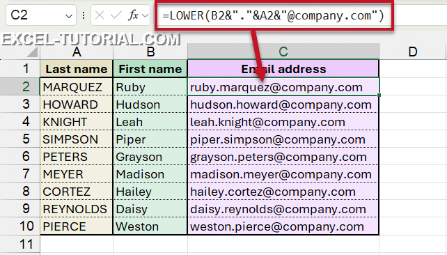
=LOWER(B2&”.”&A2&”@company.com”)
Result: ruby.marquez@company.com. Copy it down the column and the whole list is built.
Read it from the inside out: the cells are joined with the & operator, then LOWER wraps the whole expression and forces everything to lowercase in one go. No need to apply it to each piece.
Only the first letter of the first name
Many companies use a shorter form: the first initial, then the last name. Keep only the first character of the first name with LEFT:
=LOWER(LEFT(B2,1)&”.”&A2&”@company.com”)
Result: r.marquez@company.com. LEFT(B2,1) returns the first letter of the first name, and the rest of the formula remains unchanged.

Without a formula: Flash Fill
Excel can also build the addresses for you, with no formula at all:
- Type the first two addresses by hand in C2 and C3: ruby.marquez@company.com and hudson.howard@company.com. Two examples help Excel understand the pattern.
- Select the cells to fill, here C2:C10.
- Go to Home > Fill > Flash Fill (or press Ctrl + E).

Excel follows the pattern of your examples and fills the rest of the column. It also works for the short form: type r.marquez@company.com and Flash Fill uses the initial.
⚠️ The difference with the formula: Flash Fill writes values, not formulas. If a name changes, or if you add a new person, nothing updates: you have to run Flash Fill again.⚠️ Use it for a one-off list, and the formula for a list that changes. More examples in Extract text with AI in Excel with FlashFill.
The two things that will break it
Invisible spaces
A list exported from another system almost always carries trailing spaces. If the cell contains “Ruby “ with a space at the end, you get ruby .marquez@company.com: an address that will bounce, and that looks perfectly normal on screen. Wrap each cell in TRIM:
=LOWER(TRIM(B2)&”.”&TRIM(A2)&”@company.com”)
Accents and special characters
LOWER handles capital letters, but it does not touch accents. Many names keep them, for example Vietnamese names: Thảo Trần gives thảo.trần@company.com, which most mail systems refuse.
SUBSTITUTE replaces one character at a time:
=SUBSTITUTE(SUBSTITUTE(A2,”ầ”,”a”),”ả”,”a”)
⚠️ One SUBSTITUTE per character quickly makes a very long formula. Above three or four special characters, clean the names in a helper column first, then build the address from it: the formula stays readable, and you can check what it changed.
Compound names need the same care: De La Cruz contains spaces, and Mary-Jane a hyphen. Decide on a rule (remove them, or keep the hyphen) and apply it with SUBSTITUTE.
And the duplicates
Two people called John Smith give the same address. Before sending anything, run the generated column through a duplicate check. It takes ten seconds, and it is the one mistake nobody catches by reading.
Now practise
Joining a first name and a last name is the base of every email address. Try it in a real spreadsheet, free and corrected as you type: six steps, with the & operator, then CONCAT, then TEXTJOIN.


