Many people now use AI to build their Excel formulas. But everyone has had the experience: the result doesn’t always meet expectations, or it creates more problems than it solves 😡🫤
Here are the points to take into account to build your prompts well, and get simple and consistent results.
1. Choose your verb carefully
The AI reads every word of your prompt, and the verb decides the type of function it will choose. Compare these two requests:
I want to find the price of the product P-104.The verb find leads the AI to a lookup function, like XLOOKUP:
=XLOOKUP(“P-104”,A2:A50,C2:C50)
I want to know if the price of the product P-104 is above 100.The words know if lead the AI to a condition:
=IF(XLOOKUP(“P-104″,A2:A50,C2:C50)>100,”Yes”,”No”)
Same data, two different formulas. So before sending your prompt, read it again and ask yourself: does my verb say exactly what I want? Find, count, add up, know if, extract, list… each one leads to a different family of functions.
2. The formula is too complex? Ask for a simpler one
When the prompt is vague, the AI tends to give very complex answers. It often builds solutions with LET or LAMBDA, ten lines long. An expert sees immediately that something is wrong. A beginner copies the formula and can’t maintain it when the workbook changes.
⚠️This is your safeguard: when a formula looks too complex to you, it probably is. Don’t try to understand it. Ask again:
This formula is too complex.
Is there a simpler solution, or a solution with more recent functions?
Very often, the second answer is two or three times shorter. And this leads directly to the next point.
3. Ask for the new functions
An AI learns from what is already written on the web. And on the web, there are thousands of articles on SUMIF and COUNTIF, written over twenty years. So that’s what the AI suggests first.
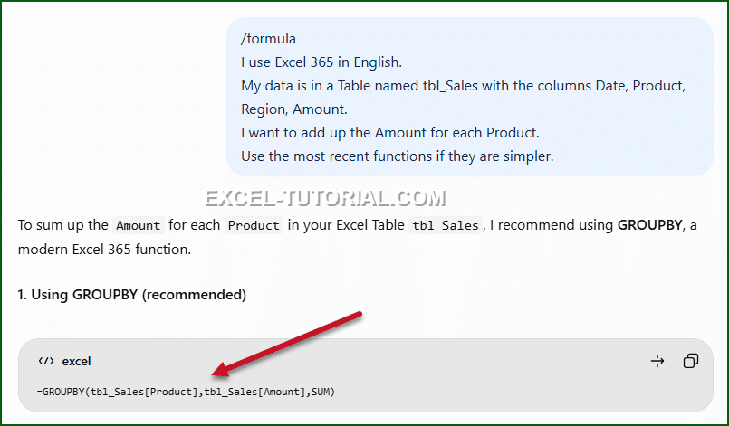
But Excel 365 has new functions that do the same job much better, and very few articles talk about them. For example, to get the total sales for each product, you used to write one SUMIF per product. Now, GROUPBY does it in one formula, and the list of products updates by itself (see GROUPBY vs SUMIF in Excel):
=GROUPBY(tbl_Sales[Product],tbl_Sales[Amount],SUM)
Same thing with FILTER, which returns all the rows that meet a condition, without any copy and paste:
=FILTER(tbl_Sales,tbl_Sales[Region]=”North”)
These functions only exist in Excel 365. So say which version you use, and ask for them:
I use Excel 365.
Use the most recent functions, like GROUPBY or FILTER, when they are simpler.
If you use Excel 2019 or 2021, say so too. The AI then avoids the functions you don’t have, and you don’t get the #NAME? error.
4. Add a command to say what you expect
This is the trick that changes everything. Start your prompt with a short command, and the AI knows immediately what type of answer you expect:
/formula→ a formula only, ready to paste in a cell/vba→ a VBA macro/powerquery→ the steps or the M code for Power Query/dax→ a DAX measure, for Power Pivot or Power BI/officescript→ a script for Excel on the web/explain→ an explanation of a formula you paste, argument by argument
For example:
/formula
Total Amount for the product Coffee in the North region.
⚠️ These commands are not official buttons of ChatGPT, Claude or Copilot. They are conventions that the AI understands, because they are short and clear. You can combine them with other instructions, like the language of your Excel:
/formula
My Excel is in French: use the French function names and semicolons as list separotors.
5. Put your data in a Table, and name the columns
Some AIs, like Claude, can read a workbook you send them. But when you ask for a formula in a chat, the AI only knows what you tell it. The best way to describe your data is to convert it into an Excel Table (Ctrl + T) and to give it a name, like tbl_Sales (see Excel Table Secrets to increase your Data Manipulation). Then give this name and the names of the columns in your prompt:
My data is in a Table named tbl_Sales.
The columns are: Date, Product, Region, Amount.
The AI then writes formulas with your real column names. They are easier to read, and they grow with your data:
=SUMIFS(tbl_Sales[Amount],tbl_Sales[Product],”Coffee”)
6. Check the column references in the answer
Many answers, from AIs and from websites, still select entire columns, like A:A or A:D. This is the worst thing to do. Your formula then works on more than one million rows instead of the few hundred you really have. The workbook becomes slow, and the headers or the empty cells can distort the result.
So limit the references to the right number of cells, or use a Table, which adjusts by itself. And say it in your prompt:
Don't use entire columns like A:A.
Limit the ranges to my data, or use the Table references.
The complete prompt
Here is what a good prompt looks like, with all the rules together:
/formula
I use Excel 365 in English.
My data is in a Table named tbl_Sales with the columns Date, Product, Region, Amount.
I want to add up the Amount for each Product.
Use the most recent functions if they are simpler.