Excel Tutorial
Excel tutorials, quizzes & AI guides — all levels
RSS
  • Online Excel Exercises
  • Training
  • Excel Tests
  • Sitemap
  • Premium Quizzes
  • Shop
  • My account

SUMIFS Function in Excel

Conditional - Intermediate Excel Skills: Tutorials and Articles
Reading time: 2 minutes
Views: 56,771

How do I use the SUMIFS function in Excel, and what is its purpose?

  1. Select the column with the value to add. Only one column must be selected.
  2. The column containing the first criterion. Select the column where the first criterion is.
  3. First criterion. Write the value of the first criterion.
  4. [Optional] The column containing the second criterion. Select the column where the second criterion is.
  5. [Optional] Second criterion. Write the value of the second criterion.
  6. …. and so on for your other criteria

=SUMIFS(Range to add, Column with the first criteria, First criteria, Column with the second criteria, Second criteria, ….)

Purpose of the SUMIFS function in Excel

The SUMIFS function in Excel helps to sum values based on multiple criteria or conditions. It allows you to filter and add up only the values that meet the specified criteria, making it a powerful tool for data analysis and reporting.

Example: What are the sales of the Category Drink in Germany

In this example, we aim to calculate the sales for the Category ‘Drink’ in Germany. Note: the data are in a Table named tbl_Sales. This makes it easier to visualize the columns selected.

In other words, we want to do a sum with 2 criteria

  • The first criterion: the Category
  • The second criterion: the Country

In this situation, how do you write the SUMIFS function? It’s easy

  1. Write the function and open the parentheses
  2. Select the column with the value to add (here, the column Total)
  3. Then, select the Category column (the first criterion)
  4. Just after, indicate the value of the criterion (here, Drink)
  5. Select the Country column
  6. And finally, write the value of the country (here, Germany)

=SUMIFS(tbl_Sales[Total],tbl_Sales[Category],”Drink”,tbl_Sales[Country],”Germany”)
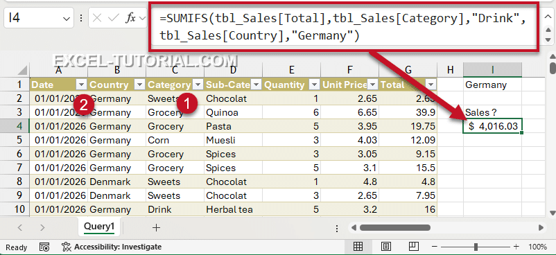
SUMIFS function to calculate the amount of drinks sales in Germany

Use references instead of the name of the criteria

Writing “Germany” inside the formula works, but the formula only answers one question. To get the sales of another country, you have to edit the formula each time.

Instead, type the country in a cell, here I1, and select this cell as the criterion. Don’t write quotes around a cell reference: the quotes are only for text typed directly in the formula.

=SUMIFS(tbl_Sales[Total],tbl_Sales[Category],”Drink”,tbl_Sales[Country],I1)

Now, if we replace Germany with Australia in the cell I1, we will return the number of sales for the Drinks in Australia 😀👍 The formula doesn’t change, only the content of the cell.
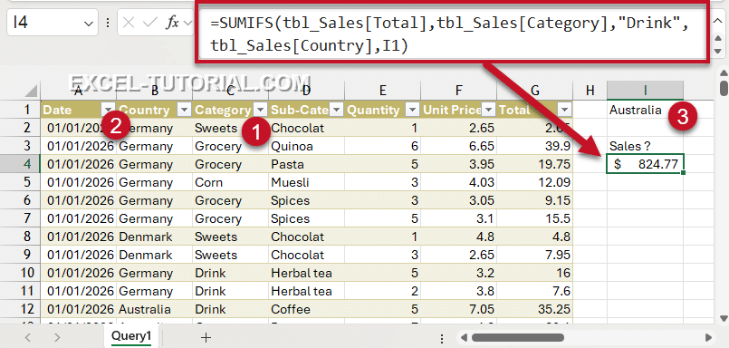
SUMIFS function with criteria as variable for the country

Build a report for all the countries

Let’s go one step further and calculate drink sales for every country at once. First, we need the list of the countries, each written only once. The UNIQUE function extracts all the different values of a column, and the SORT function puts them in alphabetical order. In the cell I4, write:

=SORT(UNIQUE(tbl_Sales[Country]))

Write the formula in one cell, and Excel fills the cells below with all the countries, from Australia to the last one. If a new country is added to the table, it automatically appears in the list.

Then, in J4, write the SUMIFS function with the cell I4 as the criterion for the country, and copy the formula down to the last country.

=SUMIFS(tbl_Sales[Total],tbl_Sales[Category],”Drink”,tbl_Sales[Country],I4)
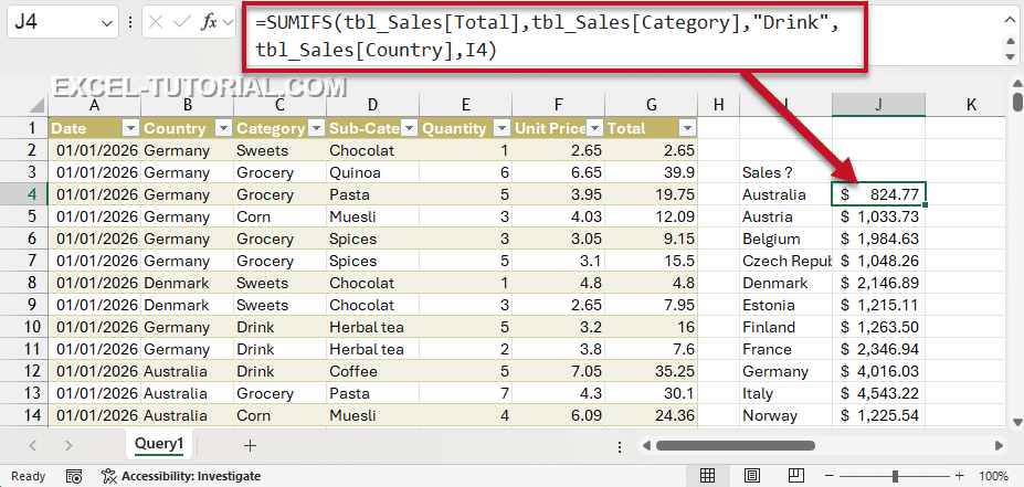
Summary of the sales for all the countries with the SUMIFS function

AND JUST LIKE THAT, you have built a report to visualize all the results for all the countries 👍👏

Related articles

  • COUNTIF, counts on a single criterion
  • COUNTIFS, counts rows for many criteria
  • How to use wildcards with COUNTIFS and SUMIFS
  • Training with the SUMIF and SUMIFS functions
  • GROUPBY vs SUMIF in Excel
  • SUMIF vs SUMIFS in Excel: The Trap of the Argument Order

Frédéric LE GUEN

Condition, most useful functions, SUMIF, SUMIFS, Top 10, UNIQUE, UNIQUE function

1 Comment

  1. Tabinda
    15/06/2022 @ 05:43

    whatever data use, request to provide for practice

    Reply

Leave a Reply Cancel reply

Your email address will not be published. Required fields are marked *

Most Viewed Posts

  • Displaying Negative Numbers in Parentheses in Excel (310,065)
  • Top 10 Excel Functions You Must Know (232,001)
  • How to make automatic calendar in Excel (212,775)
  • Dash for a zero in Excel automatically (190,813)
  • Converting a Date from YYYYMMDD to DD/MM/YYYY in Excel (171,034)
image excel exercises
Excel Exercises
image excel quizzes
Excel Quizzes

SUMIFS Function in Excel

Reading time: 2 minutes
Views: 56,771

How do I use the SUMIFS function in Excel, and what is its purpose?

  1. Select the column with the value to add. Only one column must be selected.
  2. The column containing the first criterion. Select the column where the first criterion is.
  3. First criterion. Write the value of the first criterion.
  4. [Optional] The column containing the second criterion. Select the column where the second criterion is.
  5. [Optional] Second criterion. Write the value of the second criterion.
  6. …. and so on for your other criteria

=SUMIFS(Range to add, Column with the first criteria, First criteria, Column with the second criteria, Second criteria, ….)

Purpose of the SUMIFS function in Excel

The SUMIFS function in Excel helps to sum values based on multiple criteria or conditions. It allows you to filter and add up only the values that meet the specified criteria, making it a powerful tool for data analysis and reporting.

Example: What are the sales of the Category Drink in Germany

In this example, we aim to calculate the sales for the Category ‘Drink’ in Germany. Note: the data are in a Table named tbl_Sales. This makes it easier to visualize the columns selected.

In other words, we want to do a sum with 2 criteria

  • The first criterion: the Category
  • The second criterion: the Country

In this situation, how do you write the SUMIFS function? It’s easy

  1. Write the function and open the parentheses
  2. Select the column with the value to add (here, the column Total)
  3. Then, select the Category column (the first criterion)
  4. Just after, indicate the value of the criterion (here, Drink)
  5. Select the Country column
  6. And finally, write the value of the country (here, Germany)

=SUMIFS(tbl_Sales[Total],tbl_Sales[Category],”Drink”,tbl_Sales[Country],”Germany”)

SUMIFS function to calculate the amount of drinks sales in Germany

Use references instead of the name of the criteria

Writing “Germany” inside the formula works, but the formula only answers one question. To get the sales of another country, you have to edit the formula each time.

Instead, type the country in a cell, here I1, and select this cell as the criterion. Don’t write quotes around a cell reference: the quotes are only for text typed directly in the formula.

=SUMIFS(tbl_Sales[Total],tbl_Sales[Category],”Drink”,tbl_Sales[Country],I1)

Now, if we replace Germany with Australia in the cell I1, we will return the number of sales for the Drinks in Australia 😀👍 The formula doesn’t change, only the content of the cell.

SUMIFS function with criteria as variable for the country

Build a report for all the countries

Let’s go one step further and calculate drink sales for every country at once. First, we need the list of the countries, each written only once. The UNIQUE function extracts all the different values of a column, and the SORT function puts them in alphabetical order. In the cell I4, write:

=SORT(UNIQUE(tbl_Sales[Country]))

Write the formula in one cell, and Excel fills the cells below with all the countries, from Australia to the last one. If a new country is added to the table, it automatically appears in the list.

Then, in J4, write the SUMIFS function with the cell I4 as the criterion for the country, and copy the formula down to the last country.

=SUMIFS(tbl_Sales[Total],tbl_Sales[Category],”Drink”,tbl_Sales[Country],I4)

Summary of the sales for all the countries with the SUMIFS function

AND JUST LIKE THAT, you have built a report to visualize all the results for all the countries 👍👏

Related articles

  • COUNTIF, counts on a single criterion
  • COUNTIFS, counts rows for many criteria
  • How to use wildcards with COUNTIFS and SUMIFS
  • Training with the SUMIF and SUMIFS functions
  • GROUPBY vs SUMIF in Excel
  • SUMIF vs SUMIFS in Excel: The Trap of the Argument Order
Tags: Conditionmost useful functionsSUMIFSUMIFSTop 10UNIQUEUNIQUE function

Frédéric LE GUEN

1 Comment

  1. Tabinda
    15/06/2022 @ 05:43

    whatever data use, request to provide for practice

    Reply

Leave a Reply Cancel reply

Your email address will not be published. Required fields are marked *

Contact us
About me 
Privacy Policy

© 2022 – 2026 – excel-tutorial.com. All Rights Reserved.
Excel Tutorial is managed by majordome du net

Contact us
About me 
Privacy Policy

© 2022 – 2026 – excel-tutorial.com. All Rights Reserved.
Excel Tutorial is managed by majordome du net