Excel Tutorial
Excel tutorials, quizzes & AI guides — all levels
RSS
  • Online Excel Exercises
  • Training
  • Excel Tests
  • Sitemap
  • Premium Quizzes
  • Shop
  • My account

SUMIF vs SUMIFS in Excel: The Trap of the Argument Order

Conditional
Reading time: 2 minutes
Views: 19

SUMIF and SUMIFS both add up values that meet a condition. Their names differ by one letter, but their arguments are not written in the same order. To understand why, let’s start with SUMIF.

SUMIF: the column to add comes last

SUMIF needs three arguments, always in this order: the column where you look for the condition, the condition, and the column to add, in last position. To add up the sales of the Drink category:

=SUMIF(tbl_Sales[Category],”Drink”,tbl_Sales[Total])
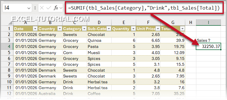
SUMIF function to calculate the sales of the drinks

Swap the two columns: no error, but no result

Now, let’s swap the column to test and the column to add:

=SUMIF(tbl_Sales[Total],”Drink”,tbl_Sales[Category])

Excel accepts the formula without any error message, but it returns 0, and it’s correct!
Excel looked for the word “Drink” in the Total column, found only numbers, and added nothing. On a report with dozens of totals, this kind of zero goes unnoticed very easily.
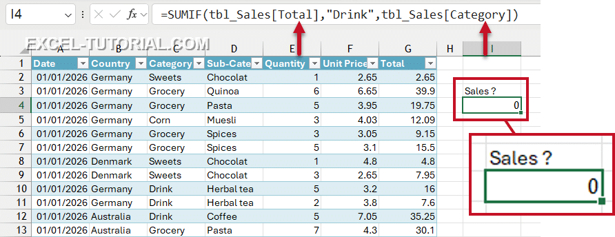
Wrong SUMIF function construction

💡 So keep this order in mind: with SUMIF, the column to add is at the end. This is exactly what changes with SUMIFS.

SUMIFS: the column to add comes first

With SUMIFS, the column to add moves to the first position. Then come the pairs “column to test, condition”. Here is the same calculation as above:

=SUMIFS(tbl_Sales[Total],tbl_Sales[Category],”Drink”)

  • SUMIF: the column to test, the condition, then the column to add (3rd and last argument).
  • SUMIFS: the column to add first, then the pairs “column to test, condition”.

Try it right now

Write your own SUMIF formulas on a sales table: totals by salesperson, by region and by product, in 6 steps, free and corrected as you type:

SUMIF Exercise - Total sales by salesperson, region or product

Total up a sales portfolio by salesperson, region and product using SUMIF, both with a fixed value and with a cell reference — 6 guided steps.

=SUMIF( criteria_range , "criteria" , sum_range )

1 / 6

You have a portfolio of 15 sales with the salesperson, the client, the region, the product and the amount.
In G2, calculate the total revenue of Martin. Type the name in full inside the formula.

SUMIF Sales — Q1 · 569

=SUMIF(A2:A16,"Martin",E2:E16)

=SUMIF( criteria_range , cell , sum_range )

2 / 6

In G2, calculate the total revenue of Dubois. Cell G1 holds the name of the salesperson — use that cell reference.

SUMIF Sales — Q2 · 570

=SUMIF(A2:A16,G1,E2:E16)

=SUMIF( criteria_range , "criteria" , sum_range )

3 / 6

Total revenue for the North region

SUMIF Sales — Q3 · 571

=SUMIF(C2:C16,"North",E2:E16)

=SUMIF( criteria_range , cell , sum_range )

4 / 6

In G2, calculate the total revenue of the South region. Cell G1 holds the criteria — use that reference.

SUMIF Sales — Q4 · 572

=SUMIF(C2:C16,G1,E2:E16)

=SUMIF( criteria_range , "criteria" , sum_range )

5 / 6

Total revenue for Pro License

SUMIF Sales — Q5 · 573

=SUMIF(D2:D16,"Pro License",E2:E16)

=SUMIF( criteria_range , cell , sum_range )

6 / 6

In G2, calculate the total revenue generated by Training. Cell G1 holds the criteria — use that reference.

SUMIF Sales — Q6 · 574

=SUMIF(D2:D16,G1,E2:E16)

Your score is

0%

A bit of history: why the order changed

SUMIF is one of Excel’s oldest functions. It was designed for a single condition, so the column to add could sit quietly at the end, and it is even optional.

SUMIFS only appeared in Excel 2007, together with COUNTIFS and AVERAGEIFS. It accepts up to 127 conditions, so Excel can’t know where the list of arguments ends. The only fixed place left for the column to add was the first one.

Microsoft could not change SUMIF without breaking millions of existing workbooks. So both syntaxes live side by side, and the same inversion exists between AVERAGEIF and AVERAGEIFS.

The habit that avoids the error

💡 Always use SUMIFS, even with a single condition. You only have one syntax to remember, the same as COUNTIFS and AVERAGEIFS. And when you need a second condition, just add a pair at the end:

=SUMIFS(tbl_Sales[Total],tbl_Sales[Category],”Drink”,tbl_Sales[Country],”Germany”)
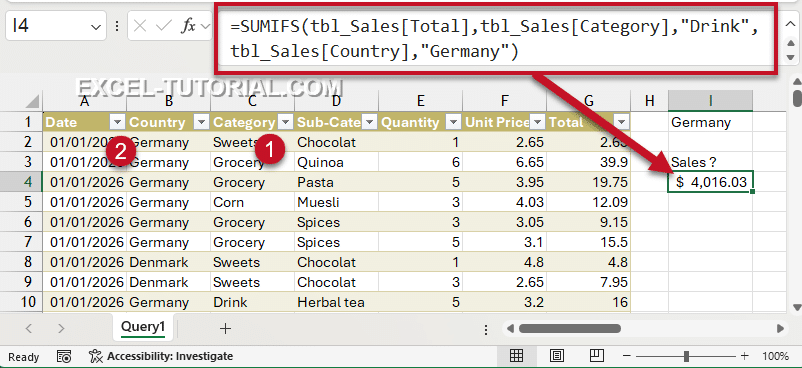
SUMIFS function to calculate the amount of drinks sales in Germany

Related Articles

  • SUMIFS Function in Excel
  • How to Use the SUMIF Function in Excel
  • Solve SUMIF Exercise: Answer Fun Questions
  • GROUPBY vs SUMIF in Excel
  • Training with the SUMIF and SUMIFS functions

Frédéric LE GUEN

Condition, SUMIF, SUMIFS

Leave a Reply Cancel reply

Your email address will not be published. Required fields are marked *

Most Viewed Posts

  • Displaying Negative Numbers in Parentheses in Excel (310,065)
  • Top 10 Excel Functions You Must Know (232,001)
  • How to make automatic calendar in Excel (212,775)
  • Dash for a zero in Excel automatically (190,813)
  • Converting a Date from YYYYMMDD to DD/MM/YYYY in Excel (171,034)
image excel exercises
Excel Exercises
image excel quizzes
Excel Quizzes

SUMIF vs SUMIFS in Excel: The Trap of the Argument Order

Reading time: 2 minutes
Views: 19

SUMIF and SUMIFS both add up values that meet a condition. Their names differ by one letter, but their arguments are not written in the same order. To understand why, let’s start with SUMIF.

SUMIF: the column to add comes last

SUMIF needs three arguments, always in this order: the column where you look for the condition, the condition, and the column to add, in last position. To add up the sales of the Drink category:

=SUMIF(tbl_Sales[Category],”Drink”,tbl_Sales[Total])

SUMIF function to calculate the sales of the drinks

Swap the two columns: no error, but no result

Now, let’s swap the column to test and the column to add:

=SUMIF(tbl_Sales[Total],”Drink”,tbl_Sales[Category])

Excel accepts the formula without any error message, but it returns 0, and it’s correct!
Excel looked for the word “Drink” in the Total column, found only numbers, and added nothing. On a report with dozens of totals, this kind of zero goes unnoticed very easily.

Wrong SUMIF function construction

💡 So keep this order in mind: with SUMIF, the column to add is at the end. This is exactly what changes with SUMIFS.

SUMIFS: the column to add comes first

With SUMIFS, the column to add moves to the first position. Then come the pairs “column to test, condition”. Here is the same calculation as above:

=SUMIFS(tbl_Sales[Total],tbl_Sales[Category],”Drink”)

  • SUMIF: the column to test, the condition, then the column to add (3rd and last argument).
  • SUMIFS: the column to add first, then the pairs “column to test, condition”.

Try it right now

Write your own SUMIF formulas on a sales table: totals by salesperson, by region and by product, in 6 steps, free and corrected as you type:

SUMIF Exercise - Total sales by salesperson, region or product

Total up a sales portfolio by salesperson, region and product using SUMIF, both with a fixed value and with a cell reference — 6 guided steps.

=SUMIF( criteria_range , "criteria" , sum_range )

1 / 6

You have a portfolio of 15 sales with the salesperson, the client, the region, the product and the amount.
In G2, calculate the total revenue of Martin. Type the name in full inside the formula.

SUMIF Sales — Q1 · 569

=SUMIF(A2:A16,"Martin",E2:E16)

=SUMIF( criteria_range , cell , sum_range )

2 / 6

In G2, calculate the total revenue of Dubois. Cell G1 holds the name of the salesperson — use that cell reference.

SUMIF Sales — Q2 · 570

=SUMIF(A2:A16,G1,E2:E16)

=SUMIF( criteria_range , "criteria" , sum_range )

3 / 6

Total revenue for the North region

SUMIF Sales — Q3 · 571

=SUMIF(C2:C16,"North",E2:E16)

=SUMIF( criteria_range , cell , sum_range )

4 / 6

In G2, calculate the total revenue of the South region. Cell G1 holds the criteria — use that reference.

SUMIF Sales — Q4 · 572

=SUMIF(C2:C16,G1,E2:E16)

=SUMIF( criteria_range , "criteria" , sum_range )

5 / 6

Total revenue for Pro License

SUMIF Sales — Q5 · 573

=SUMIF(D2:D16,"Pro License",E2:E16)

=SUMIF( criteria_range , cell , sum_range )

6 / 6

In G2, calculate the total revenue generated by Training. Cell G1 holds the criteria — use that reference.

SUMIF Sales — Q6 · 574

=SUMIF(D2:D16,G1,E2:E16)

Your score is

0%

A bit of history: why the order changed

SUMIF is one of Excel’s oldest functions. It was designed for a single condition, so the column to add could sit quietly at the end, and it is even optional.

SUMIFS only appeared in Excel 2007, together with COUNTIFS and AVERAGEIFS. It accepts up to 127 conditions, so Excel can’t know where the list of arguments ends. The only fixed place left for the column to add was the first one.

Microsoft could not change SUMIF without breaking millions of existing workbooks. So both syntaxes live side by side, and the same inversion exists between AVERAGEIF and AVERAGEIFS.

The habit that avoids the error

💡 Always use SUMIFS, even with a single condition. You only have one syntax to remember, the same as COUNTIFS and AVERAGEIFS. And when you need a second condition, just add a pair at the end:

=SUMIFS(tbl_Sales[Total],tbl_Sales[Category],”Drink”,tbl_Sales[Country],”Germany”)

SUMIFS function to calculate the amount of drinks sales in Germany

Related Articles

  • SUMIFS Function in Excel
  • How to Use the SUMIF Function in Excel
  • Solve SUMIF Exercise: Answer Fun Questions
  • GROUPBY vs SUMIF in Excel
  • Training with the SUMIF and SUMIFS functions
Tags: ConditionSUMIFSUMIFS

Frédéric LE GUEN

Leave a Reply Cancel reply

Your email address will not be published. Required fields are marked *

Contact us
About me 
Privacy Policy

© 2022 – 2026 – excel-tutorial.com. All Rights Reserved.
Excel Tutorial is managed by majordome du net

Contact us
About me 
Privacy Policy

© 2022 – 2026 – excel-tutorial.com. All Rights Reserved.
Excel Tutorial is managed by majordome du net